- Discrete probability distribution (离散概率分布)
- Descriptive functions
- Expected value \(\mu\)
- Variance and standard deviation
- Linear transformation
- References
Discrete probability distribution (离散概率分布)
The discrete probability distribution is a type of probability distribution that shows all possible values of a discrete random variable along with the associated probabilities. In other words, a discrete probability distribution gives the likelihood of occurrence of each possible value of a discrete random variable.
Properties
A discrete probability distribution has the following properties:
- \(0 ≤ P(X = x) ≤ 1\). This implies that the probability of a discrete random variable, X, taking on an exact value, x, lies between 0 and 1.
- \(\sum P(X=x) =1\). The sum of all probabilities must be equal to 1.
Descriptive functions
There are two main functions can be used to describe a discrete probability distribution: the probability mass function (PMF) and the cumulative distribution function (CDF).
Probability mass function (PMF) (概率质量函数)
The probability mass function can be defined as a function that gives the probability of a discrete random variable, X, being exactly equal to some value, x. This function is required when creating a discrete probability distribution. The formula is given as follows:
$$P(X=x)=p(x)$$
In general, p(x) is a probability function if:
- p(x) >=0
- \[\sum p(x)=1\]
Note: If X is continuous, the counterpart of the function is called the probability density function (PDF), and is denoted f(x).
Cumulative distribution function (CDF) (累积分布函数)
The cumulative distribution function (CDF) gives the probability that a discrete random variable will be lesser than or equal to a particular value. The value of the CDF can be calculated by using the discrete probability distribution. Its formula is given as follows: \(F(x) = P(X ≤ x)\)
Expected value \(\mu\)
The expected value is often referred to as the “long-term” average or mean. This means that over the long term of doing an experiment over and over, you would expect this average.
The expected value E(X) often is denoted by the Greek letter \(\mu\). Another way to describe the expected value of X is the mean of X, \(\bar{X}\) .
For a discrete random variable X having the possible values \(x_1\), \(x_2\), …, \(x_n\), the expectation of X is defined as:
$$E(X)=x_1P(X=x_1)+...+x_nP(X=x_n)= \displaystyle\sum\limits_{j=1}^{n}x_jP(X=x_j)$$
Given that when the probabilities are all equal, the expected value of X is the mean of \(x_1\), \(x_2\), …, \(x_n\):
$$E(X)=\mu=\frac{1}{n}\displaystyle\sum\limits_{j=1}^{n}x_j$$
Variance and standard deviation
Variance \(\sigma^2\)
If X is a discrete random variable taking the values \(x_1\), \(x_2\), …, \(x_n\), and having probability denoted p(x), then the variance is given by:
$$Var(X)=\sigma^2=E[(X-\mu)^2]=\displaystyle\sum\limits_{j=1}^{n}(x_j-\mu)^2p(x_j)$$
In the case where the probabilities are all equal, the variance of X is given by:
$$Var(X)=\sigma^2=\frac{1}{n}\displaystyle\sum\limits_{j=1}^{n}(x_j-\mu)^2$$
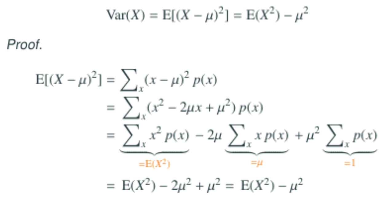
The shortcut formula f the variance is given by:
$$Var(X)=\sigma^2=E(X^2)-[E(X)]^2=E(X^2)-\mu^2$$
Proof:
Standard deviation \(\sigma\)
The standard deviation can be found by taking the square root of the variance.
Linear transformation
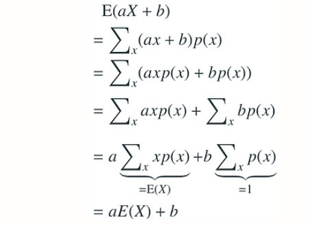
- \(E(aX + b) = aE(X) + b\) (1)
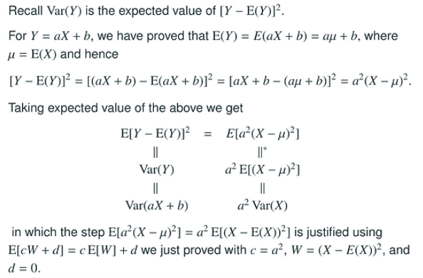
- \(Var(aX + b) = a^2 Var(X)\) (2)
Proof of (1):
Proof of (2):
References
- Probability for Dummies by Deborah Rumsey
- STAT 234 Lecture 3B Discrete Random Variables Section 3.1-3.2 of MMSA by Yibi Huang, University of Chicago
- Probability and Statistics Crash Course (Schaum’s Easy Outlines) by Murray Spiegel, John Schiller, and Alu Srinivasan