• Understanding Forward Propagation
• Steps in Forward Propagation
  • Flowchart of Forward Propagation
  • Code Implementation
• Conclusion

Understanding Forward Propagation

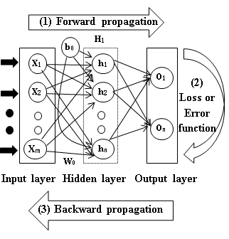
Forward propagation is the process of moving the input data through the neural network to produce an output. The input data is multiplied by the weights and biases, and passed through the activation function to produce the output. This process is repeated for each layer in the neural network until the final output is produced. The following diagram shows the computation of a feedforward neural network:

Steps in Forward Propagation

The forward propagation process in a neural network involves the following steps:

1. Initialize the network with random weights and biases.
2. Calculate the weighted sum: The input data is multiplied by the weights and biases to calculate the weighted sum.
3. Apply the activation function: The weighted sum is passed through the activation function to produce the output.
4. Repeat steps 2 and 3 for each layer: The output of one layer is used as input for the next layer, and the process is repeated until the final output is produced.
5. Output layer: Once the forward propagation process reaches the output layer of the network, the final output is calculated. In the case of a classification problem, this might involve applying a softmax function to generate probabilities for each class.

Flowchart of Forward Propagation

Code Implementation

The following Python code snippet demonstrates the forward propagation process in a neural network for recognizing handwritten digits using the MNIST dataset:

import sys, os
sys.path.append(os.pardir)
import numpy as np
from keras.datasets import mnist
from PIL import Image
import pickle

(x_train, t_train), (x_test, t_test) = mnist.load_data()
# flatten the features from 28*28 pixel to 784 wide vector
x_train = np.reshape(x_train, (-1, 784)).astype('float32')
x_test = np.reshape(x_test, (-1, 784)).astype('float32')


def img_show(img):
    pil_img = Image.fromarray(np.uint8(img))
    pil_img.show()
# img = x_train[0].reshape(28,28)
# img_show(img)

def init_network():
    with open("sample_weight.pkl",'rb') as f:
        network = pickle.load(f)
    return network

def sigmoid(x):
    return 1 / (1 + np.exp(-x))   

def softmax(x):
    x = x - np.max(x, axis=-1, keepdims=True)  
    return np.exp(x) / np.sum(np.exp(x), axis=-1, keepdims=True)

def predict(network,x):
    W1, W2, W3 = network['W1'], network['W2'], network['W3']
    b1, b2, b3 = network['b1'], network['b2'], network['b3']
    # layer 1
    A1 = np.dot(x,W1) + b1
    Z1 = sigmoid(A1)
    # layer 2
    A2 = np.dot(Z1, W2) + b2
    Z2 = sigmoid(A2)
    # output layer
    A3 = np.dot(Z2, W3) + b3
    Y = softmax(A3) # use softmax for multiple classification
    return Y

# Initialize the network
network = init_network()
x, t = x_test, t_test

accuracy_cnt = 0
batch_size = 2
for i in range(0, len(x), batch_size):
    imgs_to_pred = x[i:i+batch_size]
    y = predict(network,imgs_to_pred)
    p = np.argmax(y, axis=1) # Get the index of the label of the highest probability
    accuracy_cnt += np.sum(p==t[i:i+batch_size])
print("Accuracy:" + str(float(accuracy_cnt) / len(x)*100 )+"%")
#Accuracy:92.07%

Conclusion

In this post, we discussed the forward propagation process in a neural network. Forward propagation involves moving the input data through the network to produce an output. The input data is multiplied by the weights and biases, passed through the activation function, and the process is repeated for each layer until the final output is produced. The output layer of the network generates the final output, which can be used for classification or regression tasks. In the next post, we will discuss the backpropagation process, which is used to update the weights and biases of the network during training.