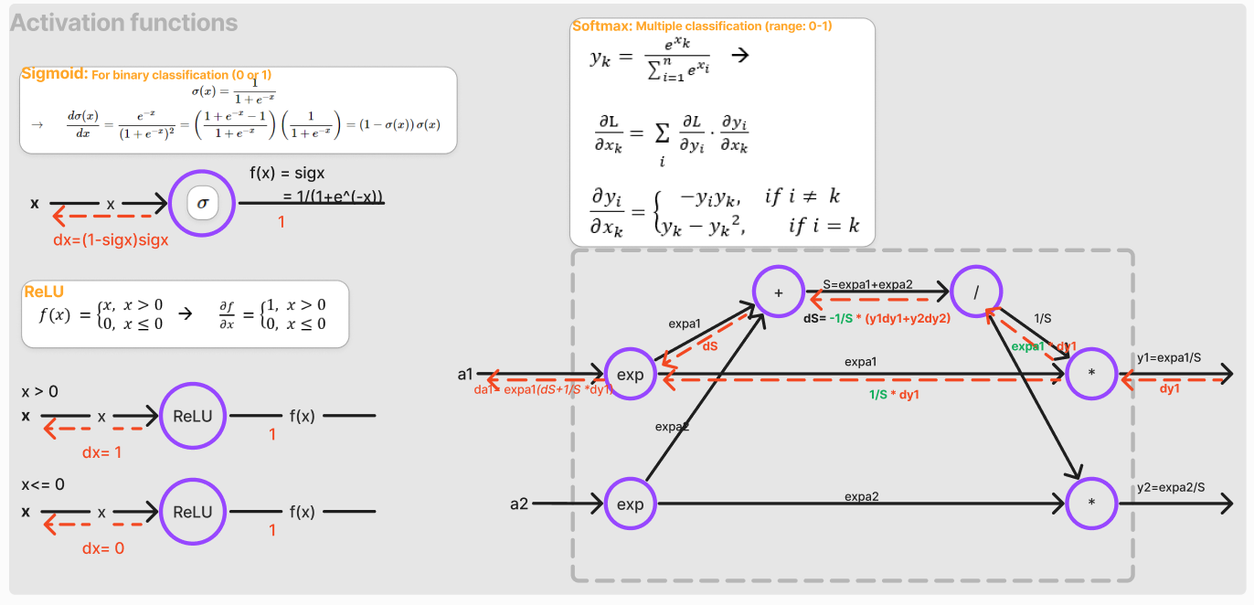
• Understanding Backpropagation
• Steps in Backpropagation
  • Flowchart of Backpropagation
• Calculating gradients
  • Computational graph method (CGM)
  • Explain CGM with a simple example
    • Calculating $ \frac{df}{df} $
    • Calculating $ \frac{df}{dz} $
    • Calculating $ \frac{df}{dq} $
    • Calculating $ \frac{df}{dx} $
    • Calculating $ \frac{df}{dy} $
  • General formula
  • Other examples
  • Patterns in gradient flow
  • Code implementation and illustration
    • Python code
    • Illustration
• Gradient Descent
  • Implementing gradient descent
    • Explicit for-loop
    • Vectorization
• Conclusion
• References

Understanding Backpropagation

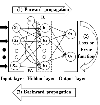
Backpropagation is the process of updating the weights and biases of a neural network during training. As it’s shown in the following diagram, backpropagation involves calculating the error between the predicted output and the actual output (shown in step 2), and then using this error to update the weights and biases of the network (step 3). This process is repeated for each layer in the network until the error is minimized.

Steps in Backpropagation

The backpropagation process in a neural network involves the following steps:

1. Calculate the error: The error between the predicted output and the actual output is calculated using a loss function.
2. Calculate the gradient: The gradient of the loss function with respect to the weights and biases is calculated using the chain rule of calculus.
3. Update the weights and biases: The weights and biases of the network are updated using the gradient descent algorithm to minimize the error.

Flowchart of Backpropagation

Calculating gradients

The gradients of the loss function with respect to the weights and biases are calculated using the chain rule of calculus. A typical method is the mathematical technique using the chain rule. This approach needs lots of matrix calculus and is prone to errors. It is not easy to implement for complex neural networks. A better approach is to use the computational graph method. This method is more intuitive and easier to implement.

Computational graph method (CGM)

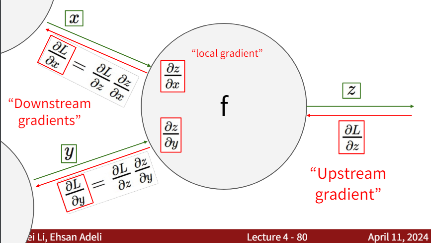
There are three main steps involved in calculating the gradients using the computational graph method:

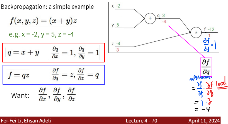
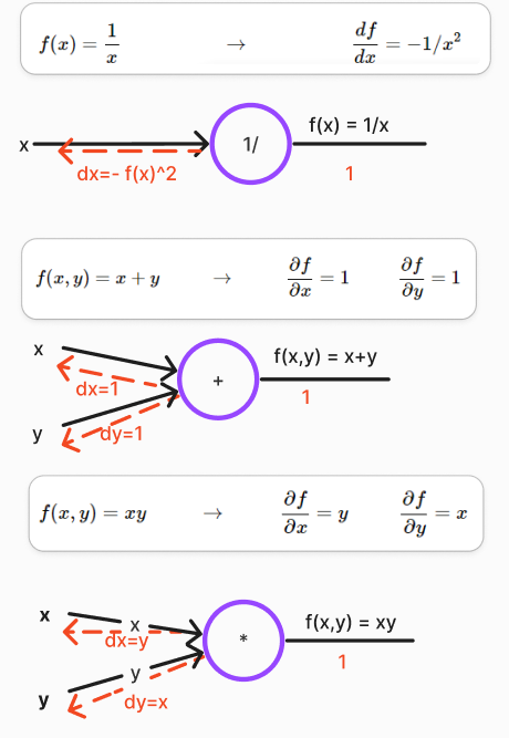
1. Calculate the local gradient: The local gradient is the derivative of the output with respect to its inputs.
2. Inherit the upstream gradient: The upstream gradient is inherited and is already calculated in the previous layer.
3. Multiply the local gradient by the upstream gradient to get the downstream gradient. This is according to the chain rule of calculus.

Note: The calculation of the gradients is done in the reverse order of the forward propagation process. Hence, the process is called backpropagation.

Explain CGM with a simple example

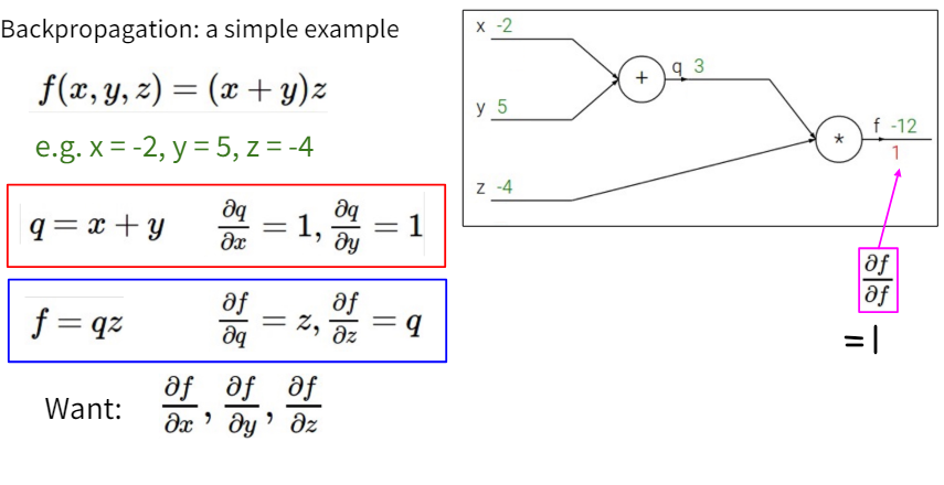
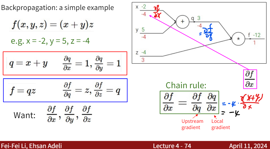
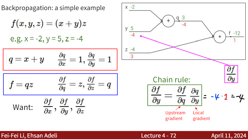
Consider a simple example as follows: \(f(x,y,z) = (x+y)z\) We want to calculate the gradient of f with respect to x, y, and z: dx, dy, dz.

Calculating $ \frac{df}{df} $

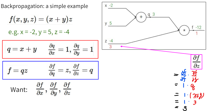
Calculating $ \frac{df}{dz} $

Calculating $ \frac{df}{dq} $

Calculating $ \frac{df}{dx} $

Calculating $ \frac{df}{dy} $

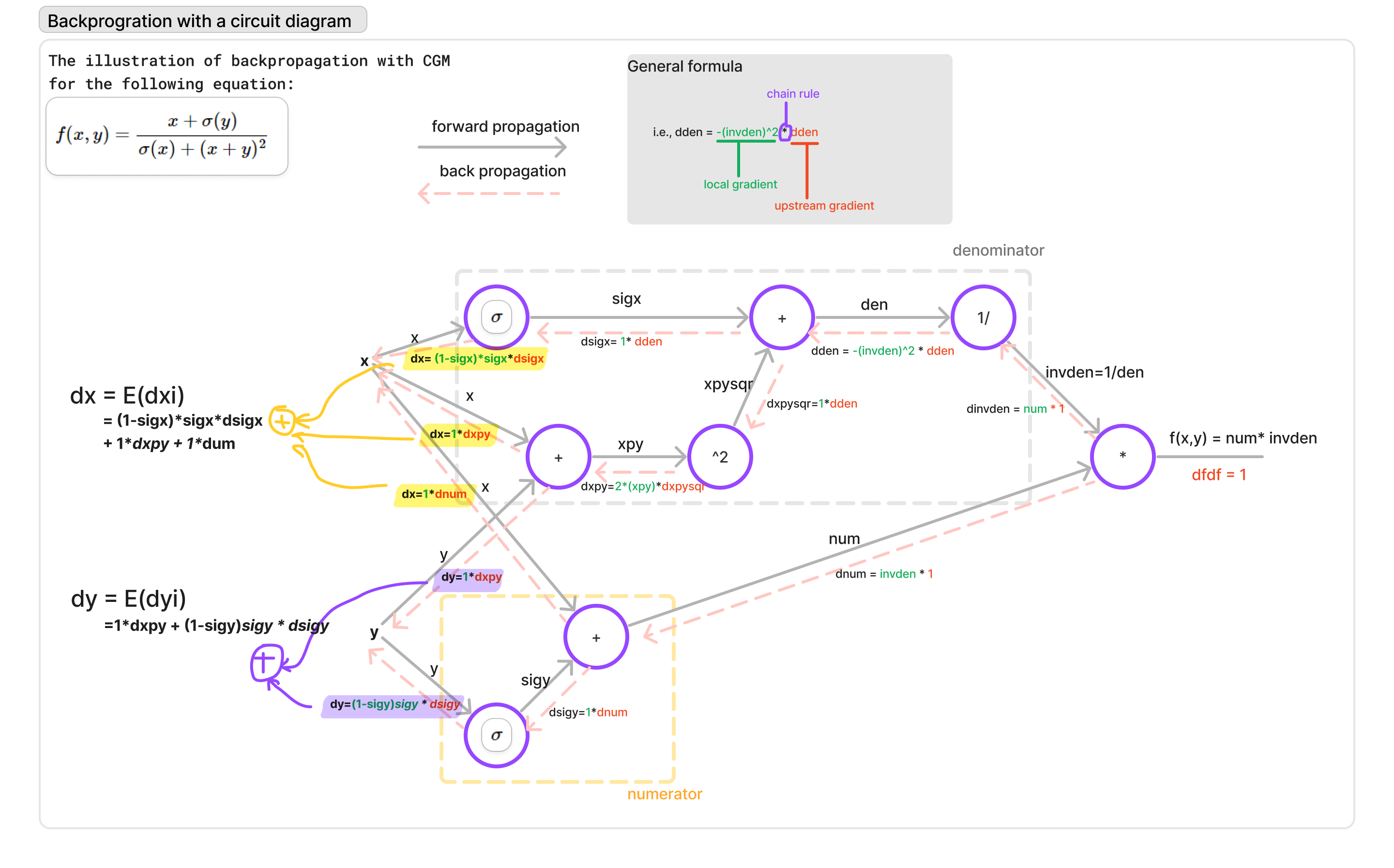
General formula

The general formula for calculating the gradients using the computational graph method is as follows:

$d_{downstream}=d_{local}\times d_{upstream}$

Other examples

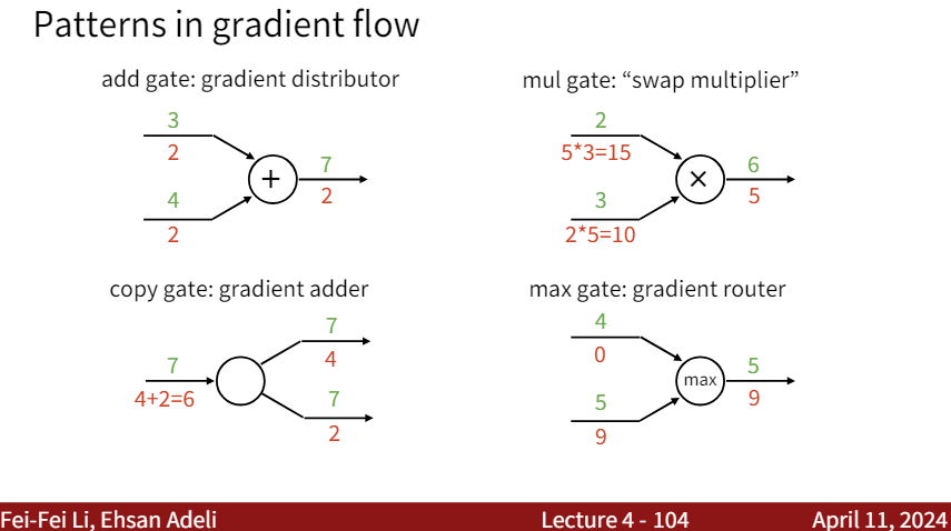
Patterns in gradient flow

Code implementation and illustration

Python code

The following Python code snippet demonstrates the backpropagation process in a neural network for a simple example:

x = 3 # example values
y = -4

# forward pass
sigy = 1.0 / (1 + math.exp(-y)) # sigmoid in numerator   #(1)
num = x + sigy # numerator                               #(2)
sigx = 1.0 / (1 + math.exp(-x)) # sigmoid in denominator #(3)
xpy = x + y                                              #(4)
xpysqr = xpy**2                                          #(5)
den = sigx + xpysqr # denominator                        #(6)
invden = 1.0 / den                                       #(7)
f = num * invden # done!                                 #(8)

# compute backpropagation
# backprop f = num * invden
dnum = invden # gradient on numerator                             #(8)
dinvden = num                                                     #(8)
# backprop invden = 1.0 / den 
dden = (-1.0 / (den**2)) * dinvden                                #(7)
# backprop den = sigx + xpysqr
dsigx = (1) * dden                                                #(6)
dxpysqr = (1) * dden                                              #(6)
# backprop xpysqr = xpy**2
dxpy = (2 * xpy) * dxpysqr                                        #(5)
# backprop xpy = x + y
dx = (1) * dxpy                                                   #(4)
dy = (1) * dxpy                                                   #(4)
# backprop sigx = 1.0 / (1 + math.exp(-x))
dx += ((1 - sigx) * sigx) * dsigx # Notice += !! See notes below  #(3)
# backprop num = x + sigy
dx += (1) * dnum                                                  #(2)
dsigy = (1) * dnum                                                #(2)
# backprop sigy = 1.0 / (1 + math.exp(-y))
dy += ((1 - sigy) * sigy) * dsigy                                 #(1)

Code reference: CS231n-optimization-2

Illustration

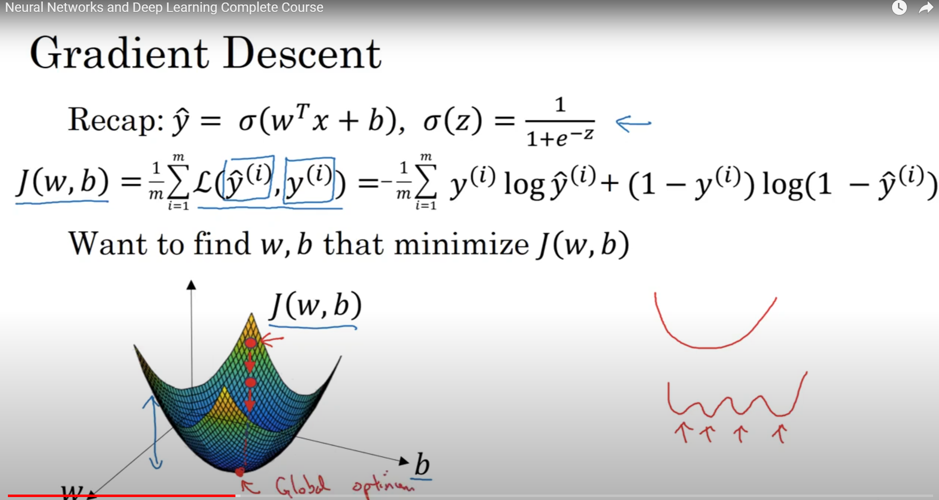
Gradient Descent

The gradient descent algorithm is used to update the weights and biases of a neural network during training.

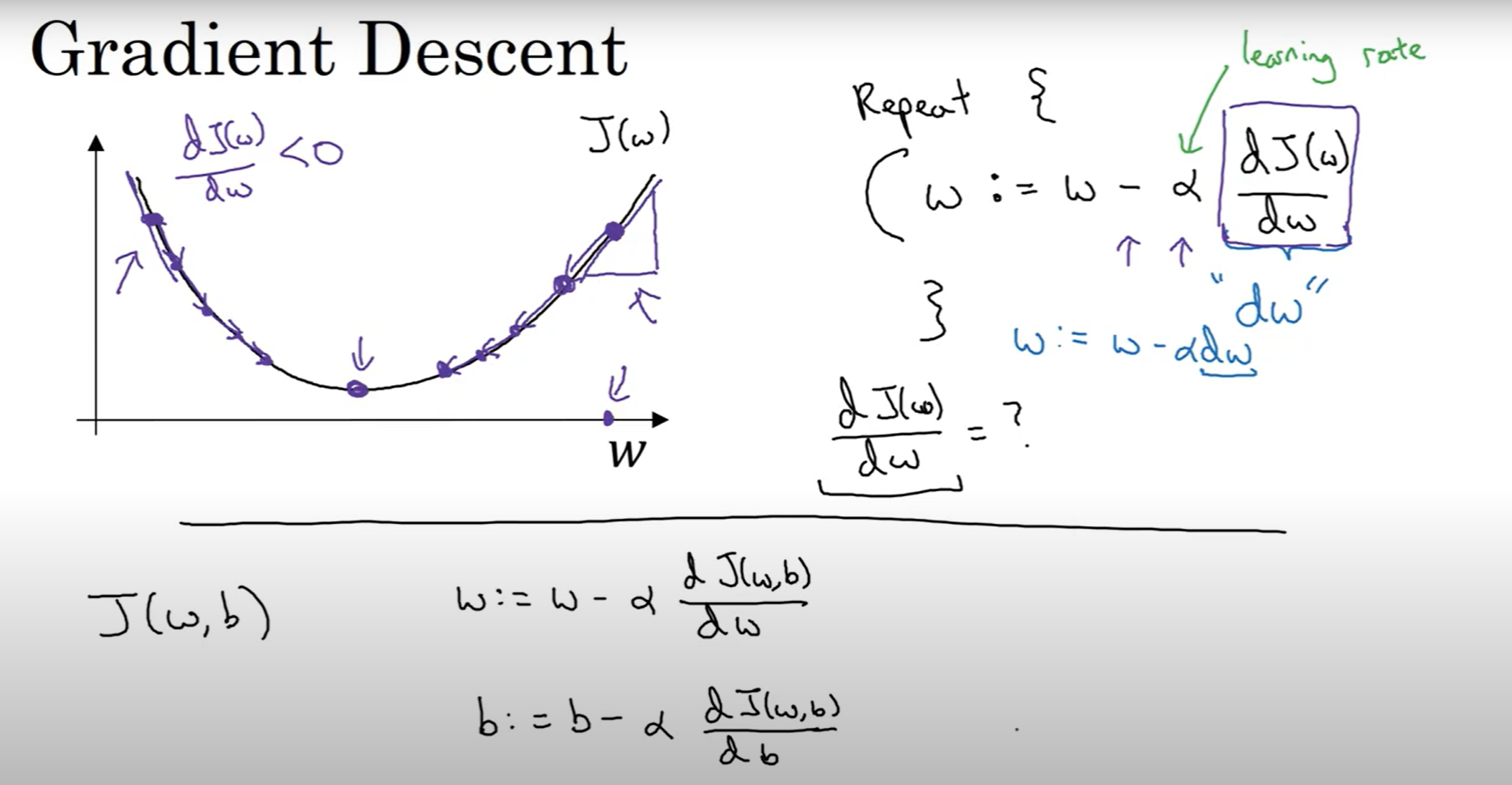
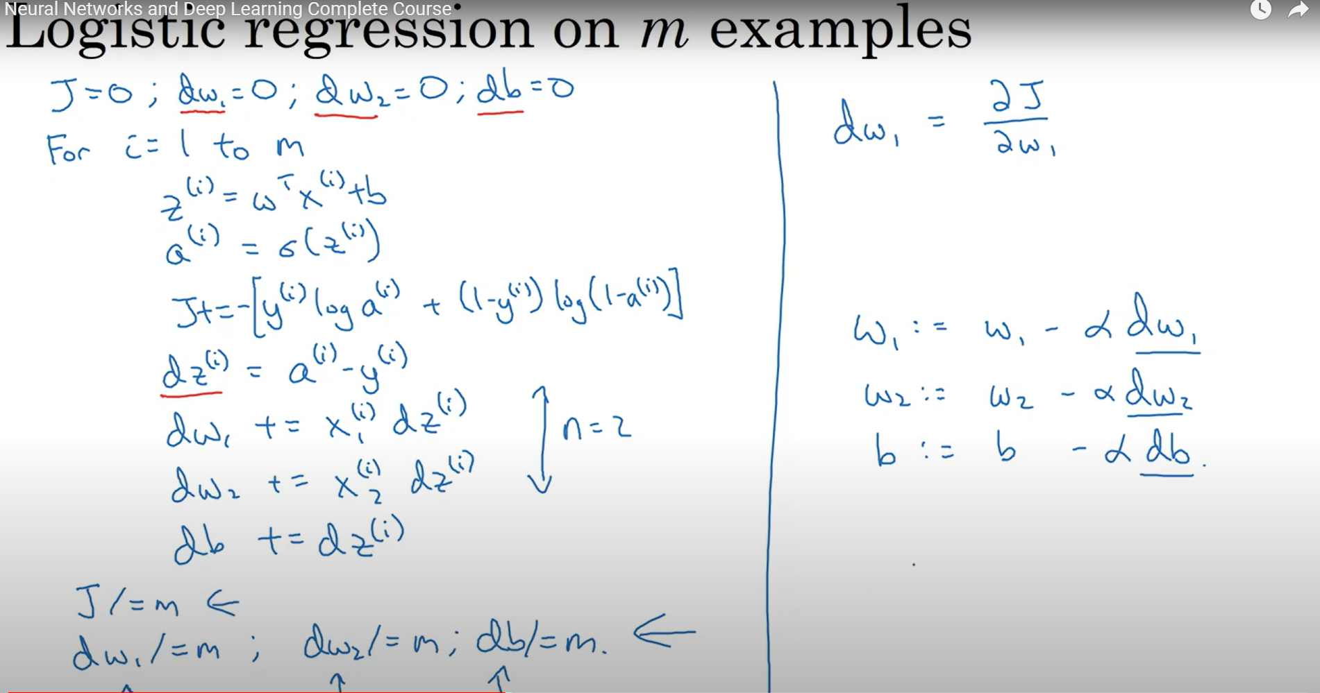
Implementing gradient descent

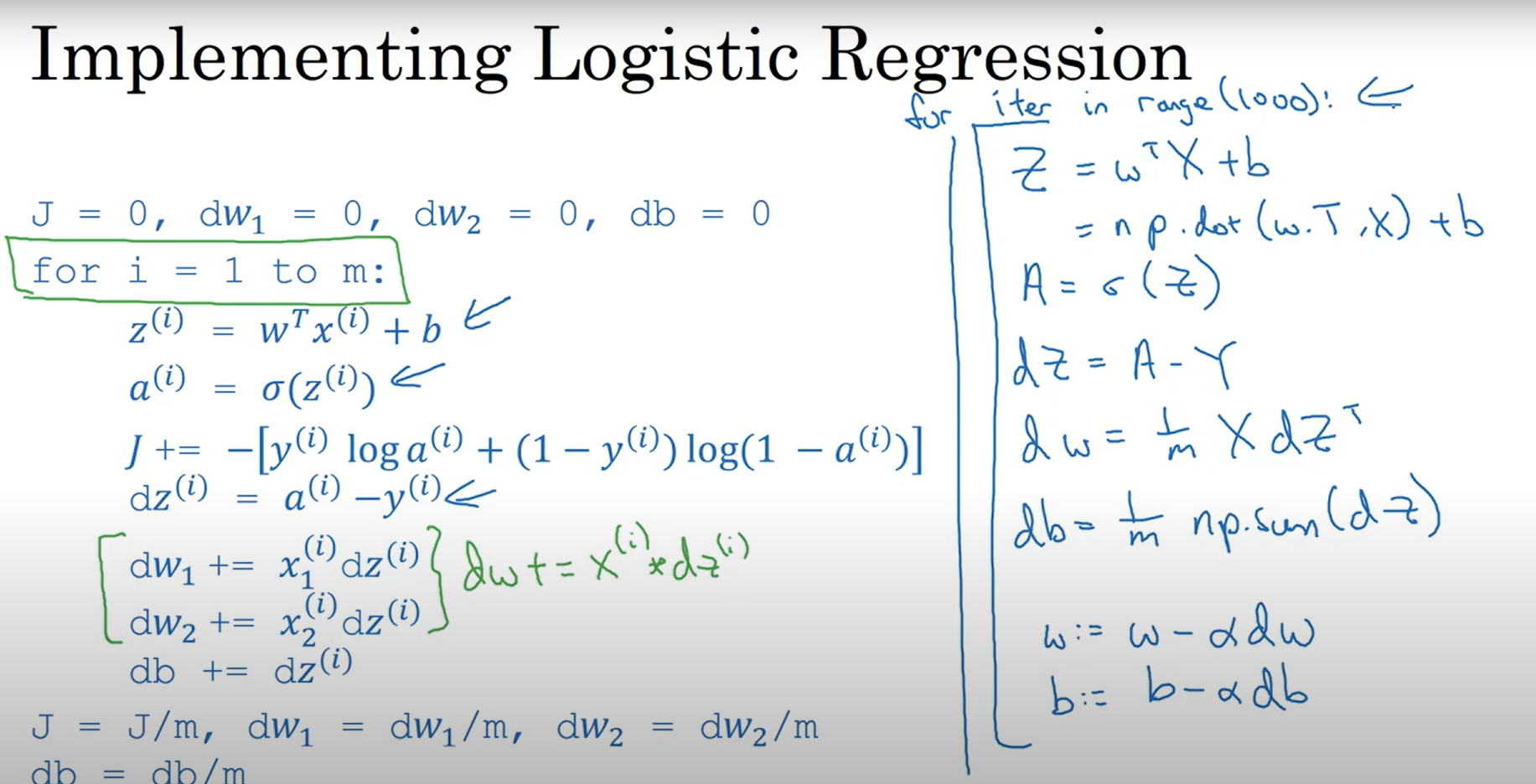
Explicit for-loop

Vectorization

Conclusion

• We developed intuition for what the gradients mean, how they flow backwards in the circuit, and how they communicate which part of the circuit should increase or decrease and with what force to make the final output higher.
• We discussed the importance of staged computation for practical implementations of backpropagation. You always want to break up your function into modules for which you can easily derive local gradients, and then chain them with chain rule. Crucially, you almost never want to write out these expressions on paper and differentiate them symbolically in full, because you never need an explicit mathematical equation for the gradient of the input variables. Hence, decompose your expressions into _stages such that you can differentiate every stage independently (the stages will be matrix vector multiplies, or max operations, or sum operations, etc.) and then backprop through the variables one step at a time._

References

• CS231n-optimization-2
• Lecture 4, CS231n 2024
• Andrew Ng’s Neural Networks and Deep Learning Course