Introduction
A Convolutional Neural Network (CNN) is a type of neural network that is designed to process data that has a grid-like topology, such as images. CNNs are widely used in computer vision tasks such as image classification, object detection, and image segmentation. In this post, we will explain the architecture of a CNN and how it works.
Convolutions
Before we dive into CNNs, let’s first understand the concept of convolutions. A convolution operation involves two functions $f$ and $g$ and the sliding of one over the other. If the functions are $f(x)$ and $g(x)$, convolution is defined as:
$$(f*g)(t)\equiv\int_{-\infty}^{\infty}f(\tau)g(t-\tau)d\tau$$
Impact of applying a filter
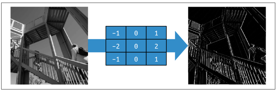
The filter $F$ is used to detect certain patterns in the input data. For example, a filter can be used to detect vertical lines, horizontal lines, or edges in an image.
For example, a filter with negative values on the left, positive values on the right, and zeros in the middle will end up removing most of the information from the image
except for vertical lines, as shown in the figure below.
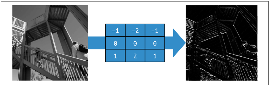
Similarly, a filter with negative values on the top, positive values on the bottom, and zeros in the middle will end up removing most of the information from the image
except for horizontal lines, as shown in the figure below.
By applying different filters to the input data, we can extract different features from the data. That’s why the output of the convolution operation is called a feature map. These features can then be used to build more complex models that can recognize objects in images.
Convolution operation
Convolution in 1D
The following figure shows a plot on the bottom and two sets of numbers labeled $f$ and $g$ on the top. The plot shows the result of the convolution of $f$ and $g$.
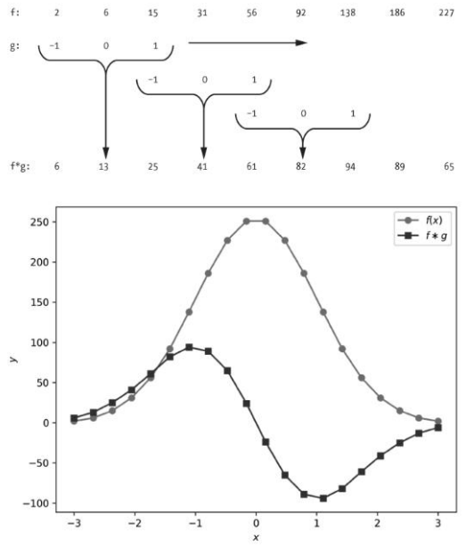
The first row lists the discrete values of the function $f$ and the second row lists the discrete values of the function $g$. The third row shows the result of the convolution of $f$ and $g$.
For example, the first element of the result, 13, is the sum of the element-wise multiplication of the first element of $f$ and the first element of $g$:
\([2, 6, 15] \circledast [-1, 0, 1] = 2\cdot (-1) + 6 \cdot 0 + 15 \cdot 1 = 13\)
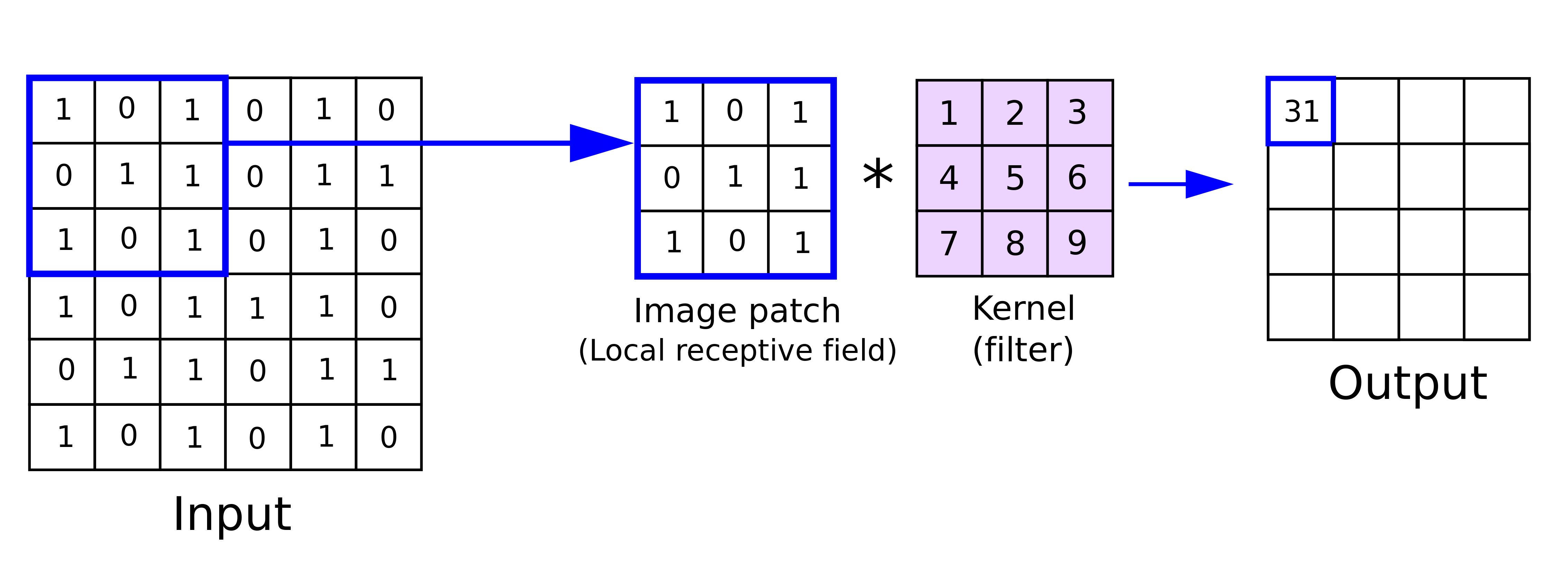
Convolution in 2D
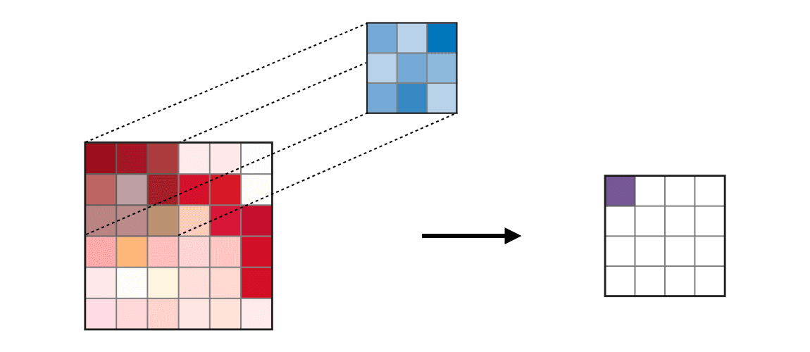
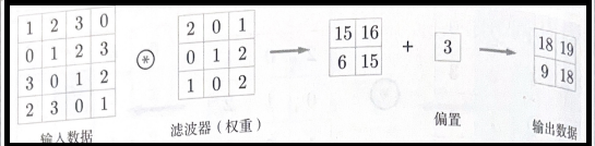
The convolution can be explained by sliding the kernel or filter, $f$, of a given strides $S$ over the input data and computing the element-wise multiplication of the slided input data and the filter and then summing the results.
When the filter is slided over the entire input data, the output matrix $O$ (aka. feature map or activation map) is produced and is considered as the output of the convolution operation. See the following illustration of the convolution operation:
 Source: https://stanford.edu/~shervine/teaching/cs-230/cheatsheet-convolutional-neural-networks
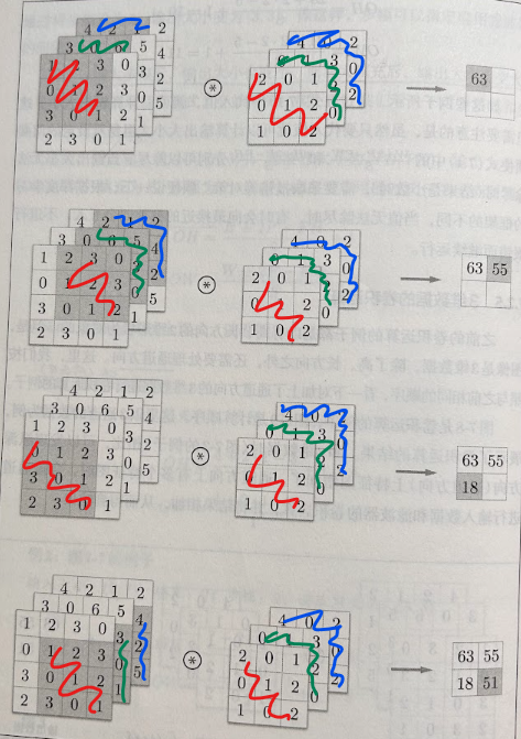
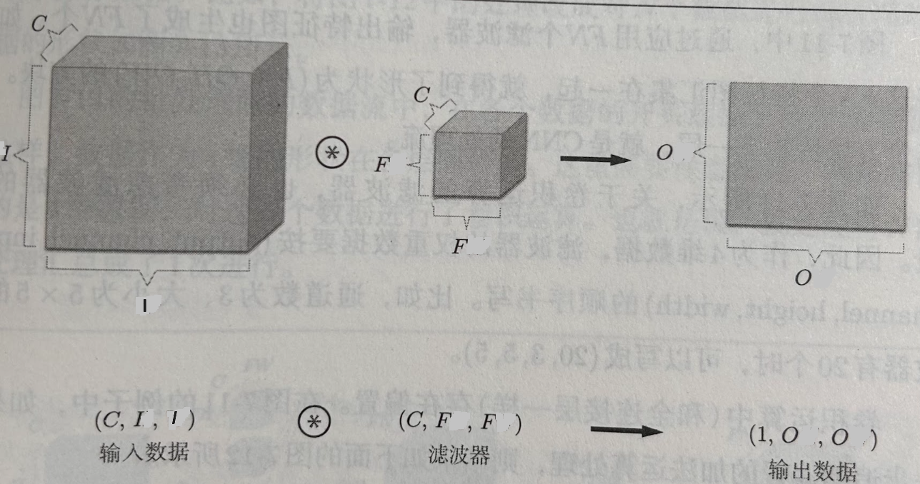
Convolution in 3D
Here we want to discuss the convolution over 3D data, such as an RGB image. The convolutions over 3D is also called convolutions over volumes. The input data of each channel is convolved with the filter of the same channel. The results are then summed to produce the output of the convolution operation.
Animation of Convolution-3D operation: Convolution-3D
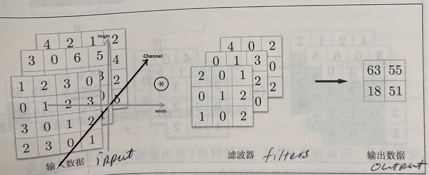
Note: The number of channels in the input data and the filter must be the same. This is because the filter is applied to each channel of the input data separately.
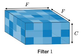
Think of the input data and the filter as 3D blocks. A filter of size $F \times F $ applied to an input containing $C$ channels is a $ F \times F \times C$ volume as shown in the following figure:
Performing convolutions on an input of size $ I \times I \times C$ with the above filter produces an output of size $ O \times O \times 1$ where:
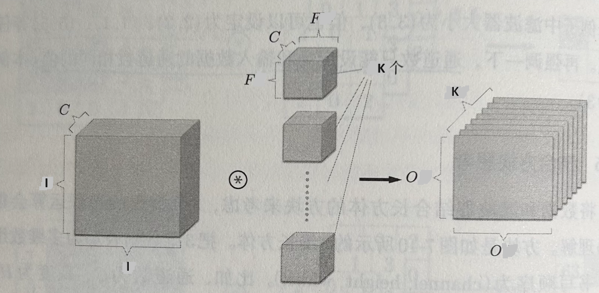
If we use $K$ filters, the output is a feature map of size $ O \times O \times K$:
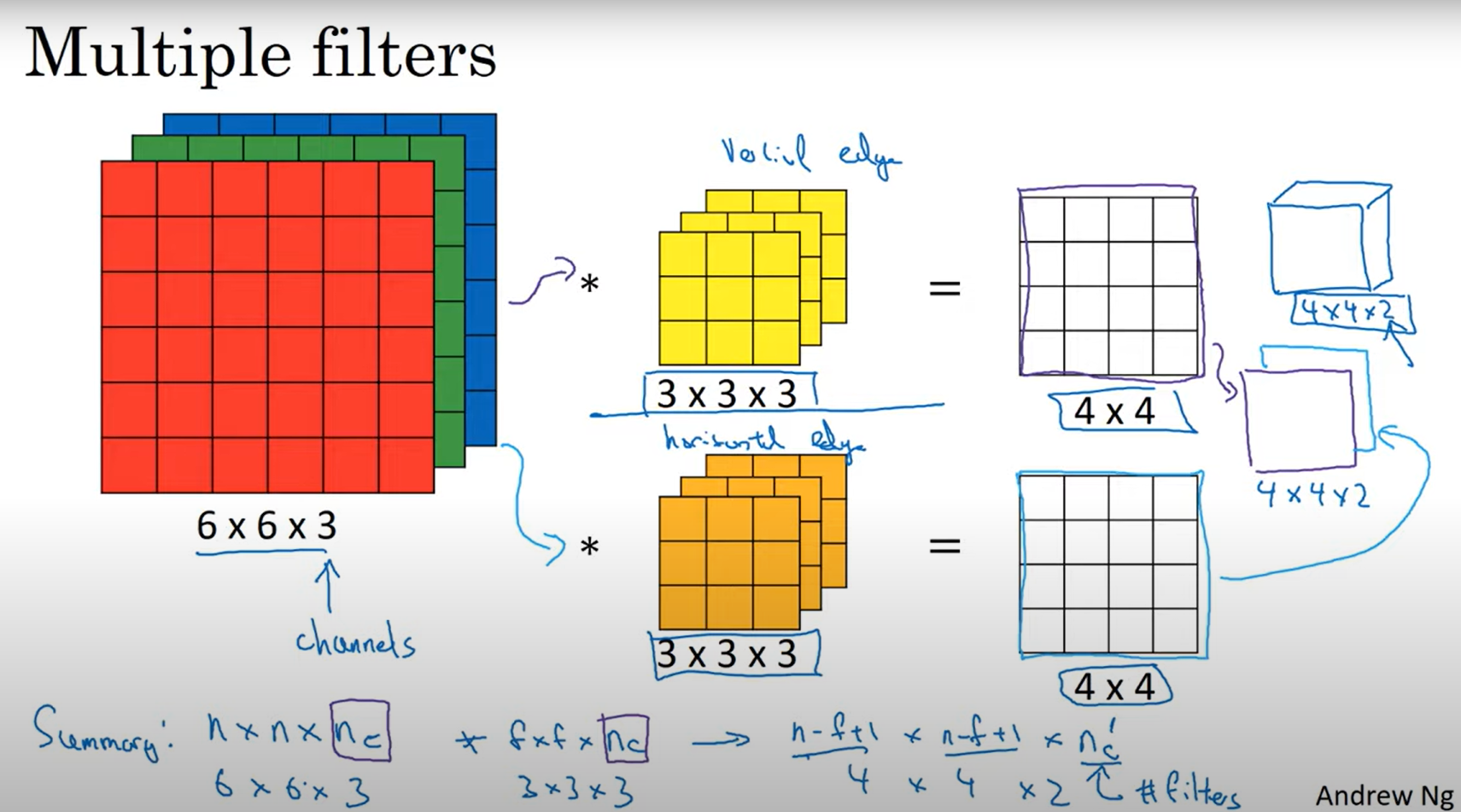
In his video, C4W1L06 Convolutions Over Volumes, Andrew Ng explains the concept of convolutions over volumes in more detail. The following
is a snippet from the video:
Filter hyperparameters
The filter hyperparameters are the parameters that define the behavior of the filter. The most important filter hyperparameters are:
- Size $F$: The size of the filter, which is usually a square matrix with dimensions $N \times N$.
- Stride $S$: The number of pixels the filter moves each time it slides over the input data.
- Padding$P$: The number of zeros added to the boundaries of the input data.
- Number of filters: The number of filters used in the convolution operation.
Weights and biases
In the context of CNNs, a filter is a weight as we discussed in the previous post on neural networks. The biases are also used in CNNs to shift the output of the convolution operation by a certain amount.
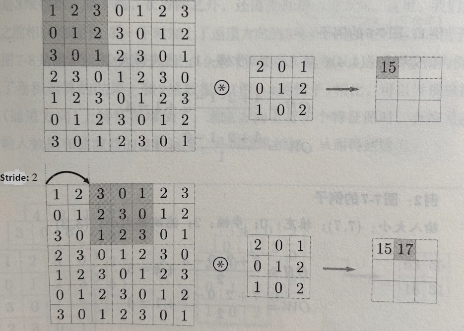
Stride $S$
For a convolutional or a pooling operation, the stride $S$ denotes the number of pixels by which the window moves after each operation. The following illustration
shows an example of a stride of 2:
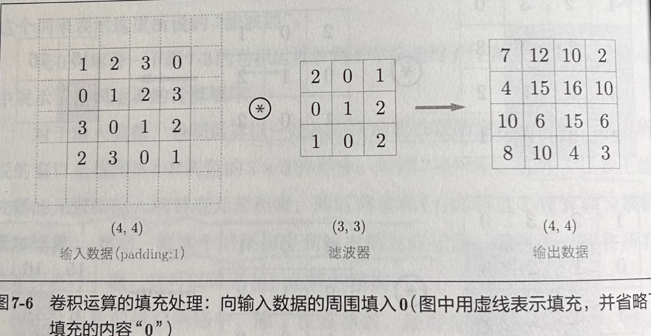
Padding $P$
Zero-padding denotes the process of adding $P$ zeroes to each side of the boundaries of the input. This value can either be manually specified or automatically set through: valid padding and same padding.
- Valid padding: No padding is added to the input data, and the filter is only applied to the parts of the input data that can be fully covered by the filter.
- Same padding: Padding is added to the input data so that the output size of the feature map is the same as the input size. See the following illustration as an example:
The relationship between the input and output sizes
As we know, the output size $O$ shrinks as the stride $S$ increases, whereas it grows as the padding $P$ increases. The following formulas can be used to calculate the output size:
\(O = \frac{I - F + P_{start} + P_{end}}{S} + 1\)
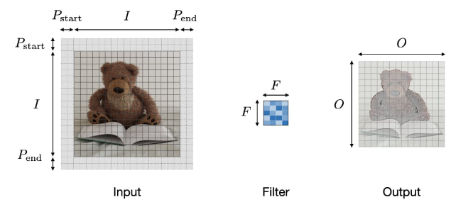
Note: often times, $P_{start}=P_{end}=P$, in which ase we can replace $P_{start} + P_{end}$ by $2P$ in the formula above and the new formula becomes: \(O = \frac{I - F + 2P}{S} + 1\)
References
- Chapter 3: Going Beyond the Basics: Detecting Features in Images, AI and Machine Learning for Coders, by Laurence Moroney, 2021, O’Reilly Media, Inc.
- CS230: Convolutional Neural Networks for Visual Recognition, Stanford University, 2021, https://stanford.edu/~shervine/teaching/cs-230/cheatsheet-convolutional-neural-networks
- C4W1L06 Convolutions Over Volumes, Andrew Ng, 2017, https://www.youtube.com/watch?v=KTB_OFoAQcc